Halos and Halo Finding in yt
Below are the slides of a talk given by Stephen Skory at the 2010 Enzo Users Conference held June 28-30 at the San Diego Supercomputer Center. This talk introduces the three different methods of finding halos available in yt, and some of the other tools in yt that can analyze and visualize halos.
The Slides
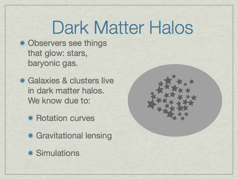
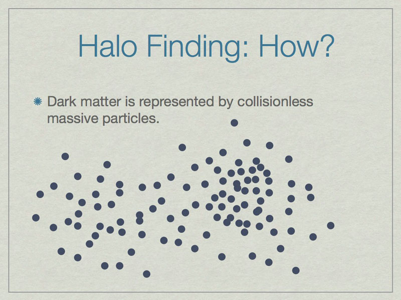
How do we know dark matter exists and surrounds galaxies? Here are some of the ways.
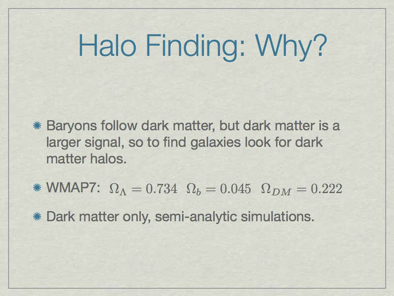
Observations look for things that glow, like stars, which live in galaxies. In simulations we want to find where the galaxies are, because that’s where the interesting things are. It is better to look for dark matter rather than stars or gas because it is a stronger signal. Also, some simulations don’t have stars or gas at all, like semi-analytic simulations.
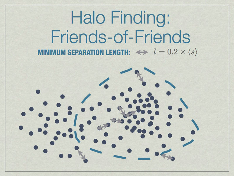
All particles closer than 0.2 of the mean inter-particle separation (s) are linked, and any all all links of particles are followed recursively to form the halo groups.
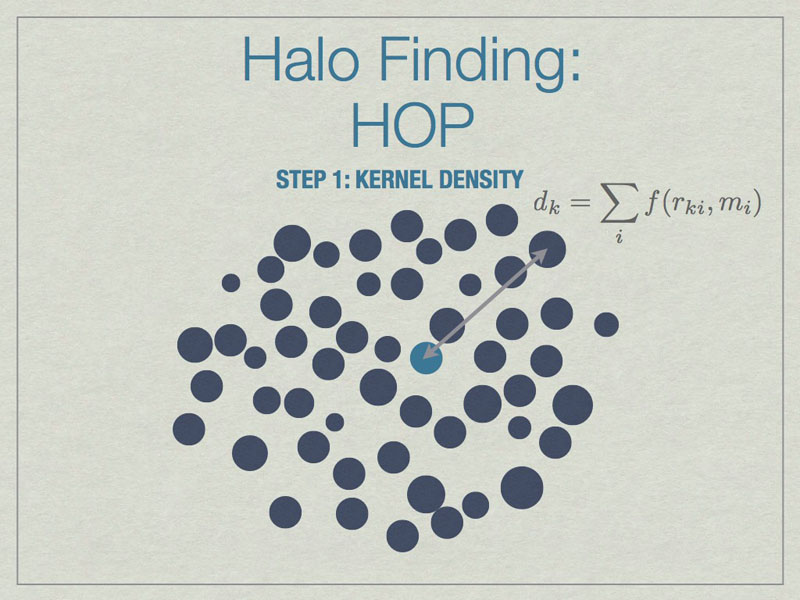
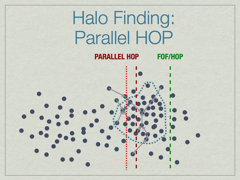
HOP starts by calculating a kernel density for each particle based on the mass of and distances to its nearest neighbors, the default is 64 of them.
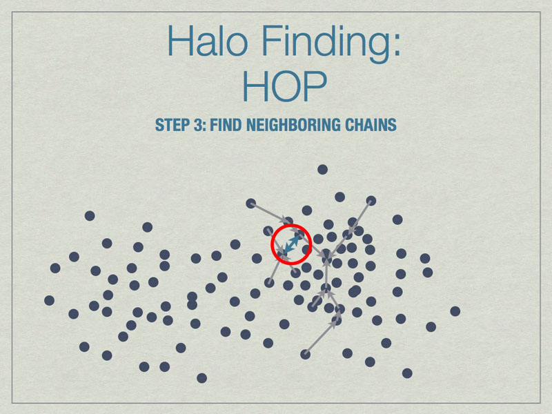
Chains are built by linking particles uphill, from a particle with lower density to one that is higher, from the set of nearest neighbors. Particles that are their own densest nearest neighbors terminate the chains. Neighborinnearest neighbors, but in different chains.
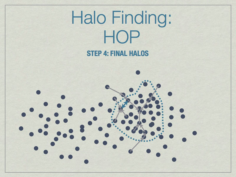
Neighboring chains are merged to build the final halos using various rules. The figure above shows the final halo enclosed by a dashed line. A few particles have been excluded from the final halo because they are underdense.
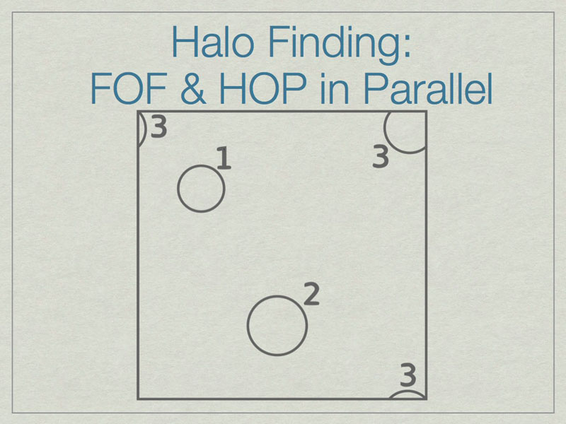
It is possible to run FOF & HOP in parallel. We start here with three halos in a volume, one of which (3) lies on the periodic boundary of the volume.
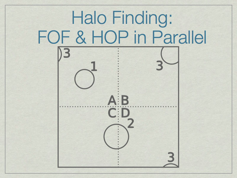
The dashed lines depict the subdivision of the full volume into subvolumes (A,B,C, and D) which define the sub-units for parallel analysis. Note that halos 2 & 3 lie in more than one subvolume.
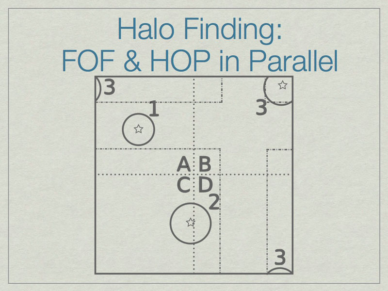
The solution is to add extra data on the faces of the subvolumes such that all halos are fully enclosed on at least one subvolume. Here subvolume C has been ‘padded’ which allows halo 2 to be fully contained in subvolume C. The centers of the halos, shown with stars, determine final ownership of halos so there is no duplication. However, this method breaks down when the halo sizes are a significant fraction of the full volume.
Parallel HOP is a fully-parallel implementation of HOP that allows both computation and memory load to be distributed using MPI parallelism.
Parallel HOP can reduce the padding by a substantial amount compared to FOF/HOP parallelism. This leads to many work- & memory-load advantages.
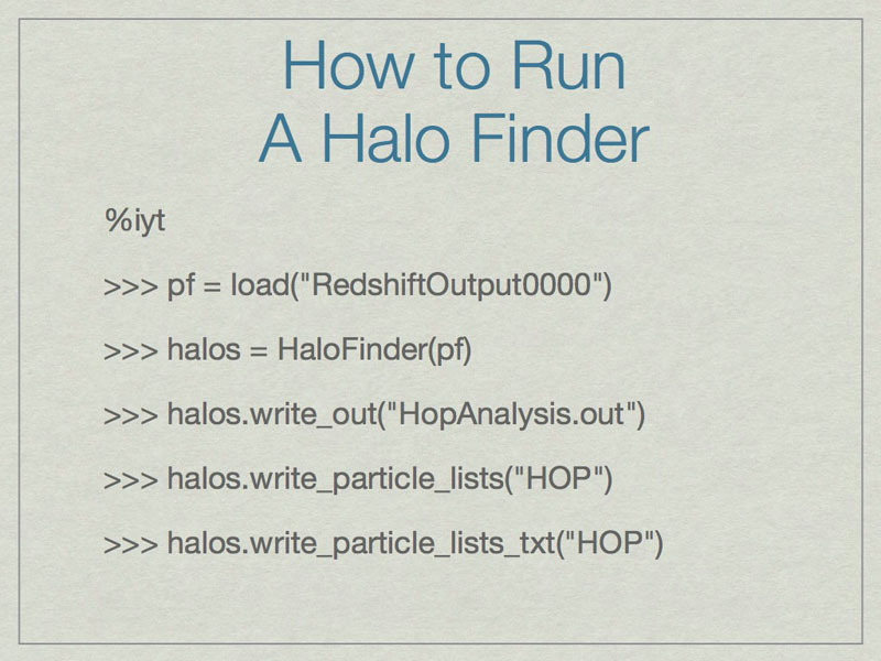
The first command builds a reference to an Enzo dataset. The second
runs HOP on the particles in the dataset and stores the result in the
halos object. The write_out command writes the halo particulars to a
text file that contains the ID, mass, center of mass, maximum radius, bulk
velocity and velocity dispersion for each halo.
write_particle_lists and write_particle_lists_txt stores the information
for the exact particles that are identified in each halo.
This shows how to find halos very simply and quickly using HOP in yt. First call ‘iyt’ from the command line. Next we reference the dataset, and then find the halos using HOP and the default settings. The next command writes out a text file with halo particulars, next the particle data for halos is written to a HDF5 file, and the last command saves a text file of where the particle halo data goes (important for parallel analysis).
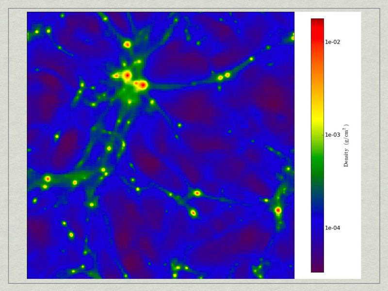
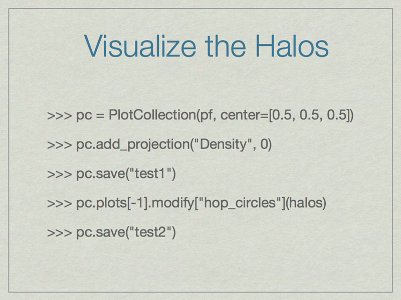
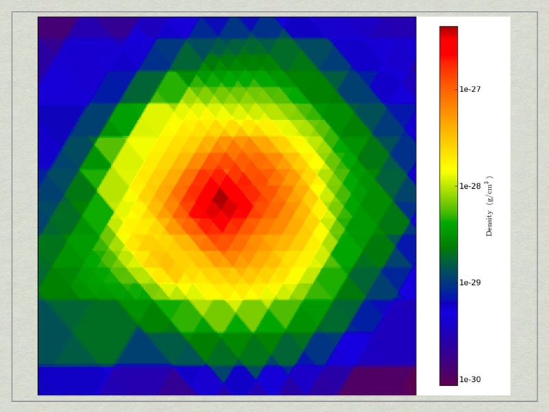
test1_Projection_x_Density.png. A density projection through a test dataset.
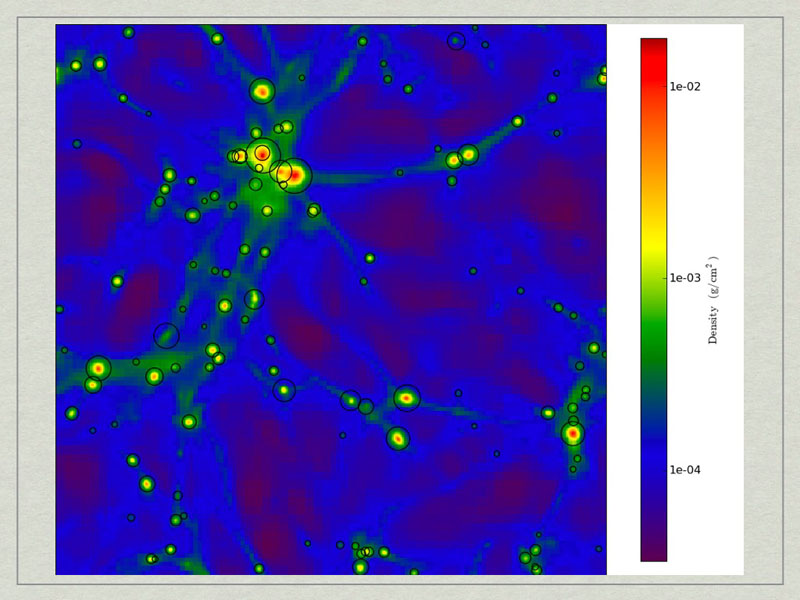
test2_Projection_x_Density.png. The halos have beecorresponds to the maximum radius of the halo.
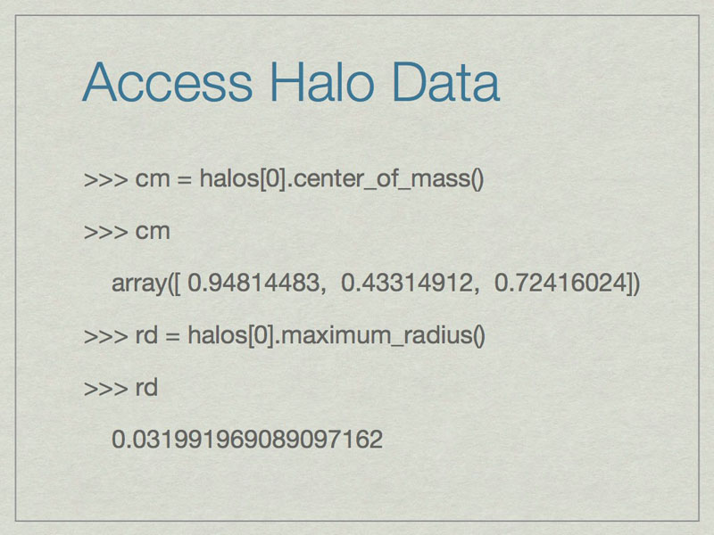
It is easy to access information about halos. All of these are in code units.
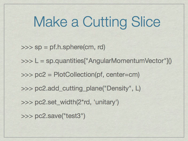
These commands will make a cutting slice through the center of the halo with normal vector oriented along the angular momentum vector of the halo.
test3_CuttingPlane__Density.pngtest3_CuttingPlane__Density.png.
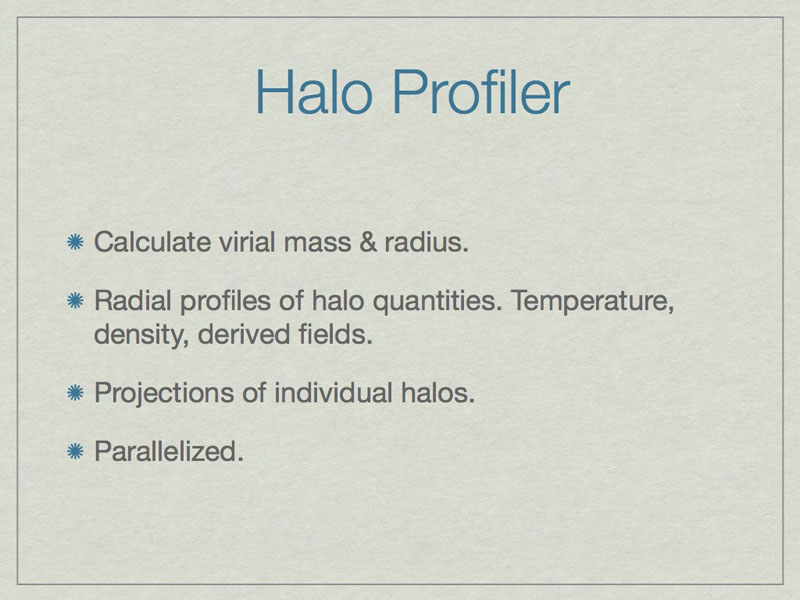
he halo profiler written by Britton Smith can analyze halos for various quantities. Given a HopAnalysis.out file, it can calculate many things on each halo.
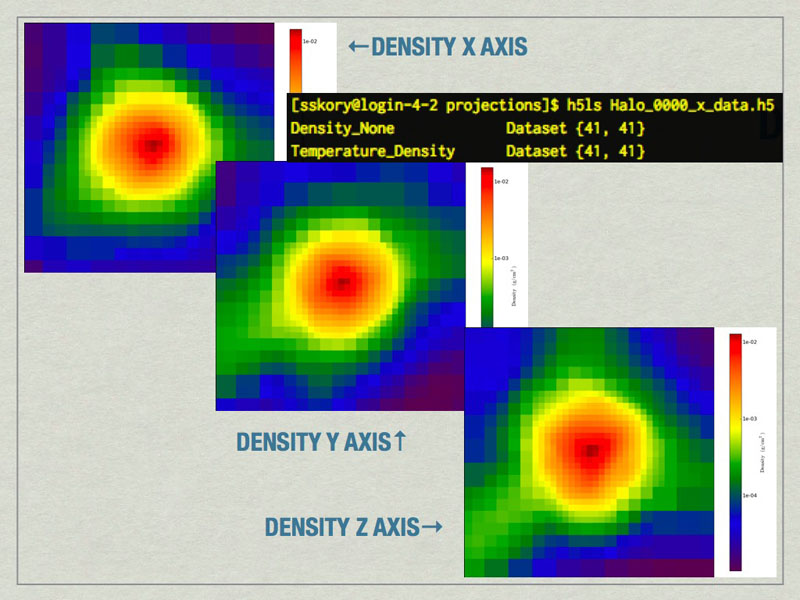
mages of the largest halo in the volume produced by the Halo Profiler. Also shown is the contents of the HDF5 files produced by the Halo Profiler.
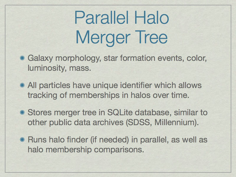
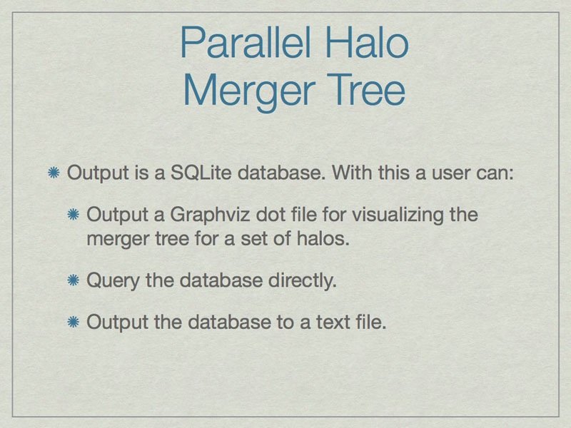
Merger trees are important when studying a halo because they affect many aspects of the halo. A merger tree tool analyzes a time-ordered series of datasets to build a comprehensive listing of the relationships between halos.
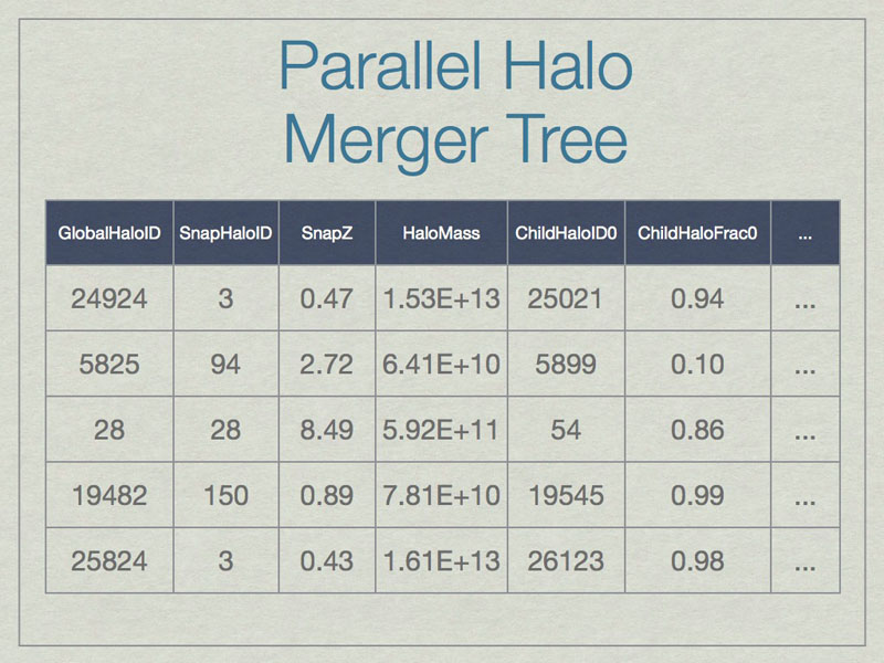
A SQL database can be thought of as a spreadsheet-like container, however entries are not ordered, unless the SQL query specifies that. This shows a few made-up example values in the database for a few real columns. Note that SnapHaloID is not unique. There are more columns in the database, but this is just an example. Columns not shown list the children for these halos.
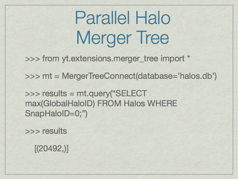
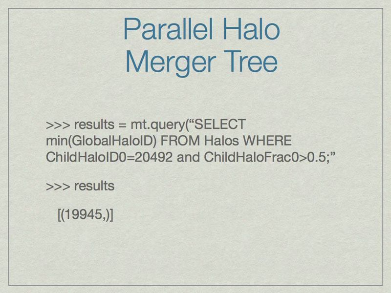
An example of how to find the GlobalHaloID for the most massive halo for the lowest redshift dataset.
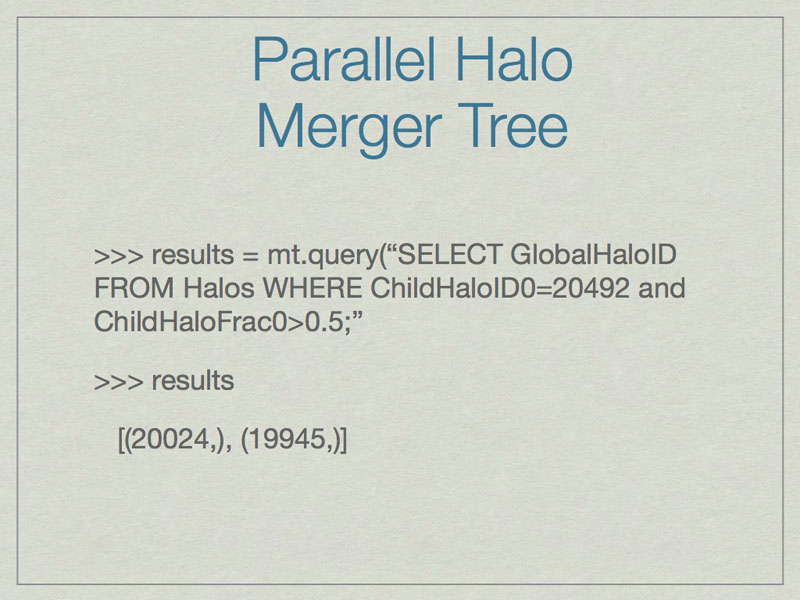
Using the output of the previous slide, an example of how to find the parents that contribute the greatest fraction of their mass to the most massive halo at the lowest redshift.
An example of how to find the most massive parent of the most massive halo at the lowest redshift.
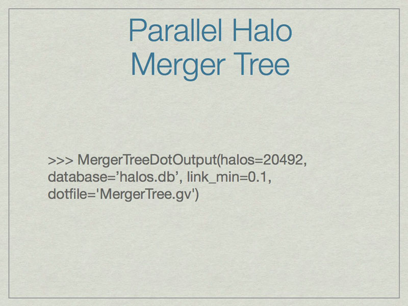
An example of how to output the full merger tree for a given halo (20492) to a graphviz file (MergerTree.gv).
Merger Tree Graphviz Example
Below is an example section of the Graphviz view of the MergerTree.gv file produced above.
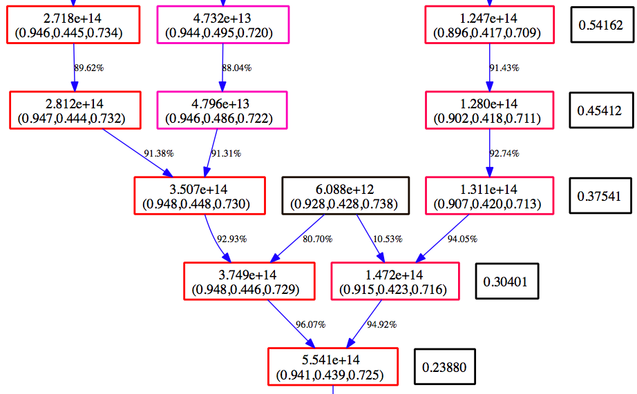
Time moves from the top to the bottom. The numbers in the black boxes give the redshift for each horizontal level of the merger tree. Each colored box corresponds to a halo that is in the merger tree for our final halo. The top number in each box gives the mass of the halo as determined by the halo finder. The second number is the center of mass for the halo in code units. The color of the box is scaled such that at each redshift, the most massive halo is red, and the smallest blue. The arrows connect a ‘parent’ halo to a ‘child’ halo, and the number next to each arrow gives the percentage of the mass of the parent halo that goes to the child halo.