Star, Black Hole and Sink Particles¶

There are many different subgrid models of star formation and feedback in the astrophysical literature, and we have included several of them in Enzo. There are also methods that include routines for black hole, sink, and Pop III stellar tracer formation. Here we give the details of each implementation and the parameters that control them. For relevant parameters please also see Star Formation and Feedback Parameters. Note that this section is particularly detailed because users are generally quite interested in the differences between the methods. Note also that multiple star particle creation routines can be used simultaneously with the StarParticleCreation parameter, as it uses a bitmask - see the parameter link above for more information.

Method 0: Cen & Ostriker
Method 1: Cen & Ostriker with Stochastic Star Formation
Method 2: Global Schmidt Law
Method 3: Population III Stars
Method 4: Sink Particles
Method 5: Radiative Stellar Clusters
Method 6: Reserved for future use
Method 7: Cen & Ostriker with no delay in formation
Method 8: Springel & Hernquist
Method 9: Massive Black Holes
Method 10: Population III stellar tracers
Method 11: Molecular Hydrogen Regulated Star Formation
Method 14: Kinetic Feedback
Restarting a Simulation With Star Formation or Feedback
Active Particle Framework
Magnetic Supernova Feedback

Method 0: Cen & Ostriker¶

Select this method by setting StarParticleCreation = 1.

Source: star_maker2.F

This routine uses the algorithm from Cen & Ostriker (1992) that creates star particles when the following six criteria are met

The gas density is greater than the threshold set in the parameter StarMakerOverDensityThreshold. This parameter is in code units (i.e. overdensity with respect to the mean matter density)
The divergence is negative
The dynamical time is less than the cooling time or the temperature is less than 11,000 K. The minimum dynamical time considered is given by the parameter StarMakerMinimumDynamicalTime in units of years.
The cell is Jeans unstable. (Note: this may not be useful depending on your physical resolution! Be very careful with this!)
The star particle mass is greater than StarMakerMinimumMass, which is in units of solar masses.
The cell does not have finer refinement underneath it.

These particles add thermal and momentum feedback to the grid cell that contains it until 12 dynamical times after its creation. In each timestep,

$M_{\rm form} &= M_0 [ (1+x_1) \exp(-x_1) - (1+x_2) \exp(-x_2) ]\\ x_1 &= (t - t_0) / t_{\rm dyn}\\ x_2 &= (t + dt - t_0) / t_{\rm dyn}$

of stars are formed, where M₀ and t₀ are the initial star particle mass and creation time, respectively.

M_ej = M_form * StarMassEjectionFraction of gas are returned to the grid and removed from the particle.
M_ej * v_particle of momentum are added to the cell.
M_form * c² * StarEnergyToThermalFeedback of energy is deposited into the cell.
M_form * ((1 - Z_star) * StarMetalYield + StarMassEjectionFraction * Z_star) of metals are added to the cell, where Z_star is the star particle metallicity. This formulation accounts for gas recycling back into the stars.

Method 1: Cen & Ostriker with Stochastic Star Formation¶

Select this method by setting StarParticleCreation = 2.

Source: star_maker3.F

This method is suitable for unigrid calculations. It behaves in the same manner as Method 1 except

No Jeans unstable check (Note: removing this check may be more broadly desirable, depending on your spatial resolution)
Stochastic star formation: Keeps a global sum of “unfulfilled” star formation that were not previously formed because the star particle masses were under StarMakerMinimumMass. When this running sum exceeds the minimum mass, it forms a star particle.
Initial star particle velocities are zero instead of the gas velocity as in Method 1.
Support for multiple metal fields.

Method 2: Global Schmidt Law¶

Select this method by setting StarParticleCreation = 4.

Source: star_maker4.F

This method is based on the Kravtsov (2003) paper that forms star particles that result in a global Schmidt law. This generally occurs when the gas consumption time depends on the local dynamical time.

A star particle is created if a cell has an overdensity greater than StarMakerOverDensityThreshold. The fraction of gas that is deposited into the star particle is dt/StarMakerMinimumDynamicalTime up to a maximum of 90% of the gas mass. Here the dynamical time is in units of years.

Stellar feedback is accomplished in the same way as Method 1 (Cen & Ostriker) but M_form = StarMakerEjectionFraction * (star particle mass).

Method 3: Population III Stars¶

Select this method by setting StarParticleCreation = 8.

Source: pop3_maker.F

This method is based on the Abel et al. (2007) paper that forms star particles that represents single metal-free stars. The criteria for star formation are the same as Method 1 (Cen & Ostriker) with the expection of the Jeans unstable check. It makes two additional checks,

The H₂ fraction exceeds the parameter PopIIIH2CriticalFraction. This is necessary because the cooling and collapse is dependent on molecular hydrogen and local radiative feedback in the Lyman-Werner bands may prevent this collapse.
If the simulation tracks metal species, the gas metallicity in an absolute fraction must be below PopIIIMetalCriticalFraction.

Stellar radiative feedback is handled by the Radiative Transfer module. By default, only hydrogen ionizing radiation is considered. To include helium ionizing radiation, set PopIIIHeliumIonization to 1. Supernova feedback through thermal energy injection is done by the Star Particle Class. The explosion energy is computed from the stellar mass and is deposited in a sphere with radius PopIIISupernovaRadius in units of pc. To track metal enrichment, turn on the parameter PopIIISupernovaUseColour.

Method 4: Sink particles¶

Select this method by setting StarParticleCreation = 16.

Source: sink_maker.C

Multiple variations on this method exist but are not being actively maintained. They require a completely different set of parameters to turn on such as BigStarFormation; see Grid_StarParticleHandler.C and Star Formation and Feedback Parameters.

Source: star_maker8.C, star_maker9.C

Method 5: Radiative Stellar Clusters¶

Select this method by setting StarParticleCreation = 32.

Source: cluster_maker.F

This method is based on method 1 (Cen & Ostriker) with the Jeans unstable requirement relaxed. It is described in Wise & Cen (2009). The star particles created with this method use the adaptive ray tracing to model stellar radiative feedback. It considers both cases of Jeans-resolved and Jeans unresolved simulations. The additional criteria are

The cell must have a minimum temperature of 10,000 K if the 6-species chemistry model (MultiSpecies == 1) is used and 1,000 K if the 9-species chemistry model is used.
The metallicity must be above a critical metallicity (PopIIIMetalCriticalFraction) in absolute fraction.

When the simulation is Jeans resolved, the stellar mass is instantaneously created and returns its luminosity for 20 Myr. In the case when it’s Jeans unresolved, the stellar mass follows the Cen & Ostriker prescription.

Method 6: Reserved for future use¶

This method is reserved for future use.

Method 7: Cen & Ostriker with no delay in formation¶

Select this method by setting StarParticleCreation = 128.

Source: star_maker7.F

This method relaxes the following criteria from the original Cen & Ostriker prescription. See Kim et al. (2011) for more details. It can be used to represent single molecular clouds.

No Jeans unstable check
No Stochastic star formation prescription that is implemented in Method 1.
If there is a massive black hole particle in the same cell, the star particle will not be created.

The StarMakerOverDensity is in units of particles/cm³ and not in overdensity like the other methods.

Method 8: Springel & Hernquist¶

Select this method by setting StarParticleCreation = 256.

Source: star_maker5.F

This method is based on the Springel & Hernquist method of star formation described in MNRAS, 339, 289, 2003. A star may be formed from a cell of gas if all of the following conditions are met:

The cell is the most-refined cell at that point in space.
The density of the cell is above a threshold.
The cell of gas is in the region of refinement. For unigrid, or AMR-everywhere simulations, this corresponds to the whole volume. But for zoom-in simulations, this prevents star particles from forming in areas that are not being simulated at high resolution.

If a cell has met these conditions, then these quantities are calculated for the cell:

Cell star formation timescale (Eqn 21 from Springel & Hernquist).

$t_0^{\ast}$ and $\rho_{\mathrm{th}}$ are inputs to the model, and are the star formation time scale and density scaling value, respectively. Note that $\rho_{\mathrm{th}}$ is not the same as the critical density for star formation listed above. $\rho$ is the gas density of the cell.

$t_{\ast}(\rho)=t_0^{\ast}\left(\frac{\rho}{\rho_{\mathrm{th}}}\right)^{-1/2}$
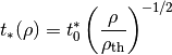
Mass fraction in cold clouds, $x$ (see Eqns. 16 and 18).

$y$ is a dimensionless quantity calculated as part of the formulation; $u_{\textrm{SN}}\equiv(1-\beta)\beta^{-1}\epsilon_{\textrm{SN}}$ is the energy released from supernovae back into the gas (note that whether or not the energy is actually returned to the gas depends on if StarFormationFeedback is turned on or not); $\beta$ is the fraction of stars that go supernova soon after formation; $\epsilon_{\textrm{SN}}$ is the energy released from a nominal supernova and is set to 4e48 ergs; and finally $\Lambda(\rho, T, z)$ is the cooling rate of the cell of gas.

$y\equiv\frac{t_{\ast}\Lambda(\rho,T,z)}{\rho[\beta u_{\mathrm{SN}}-(1-\beta)u_{\mathrm{SN}}]} x=1+\frac{1}{2y}-\sqrt{\frac{1}{y}+\frac{1}{4y^2}}$

Finally, a star particle of mass $m_{\ast}$ is created with probability $p_{\ast}$ (see Eqn. 39). For a cell, the quantity $p_{\ast}$ is calculated (below) and compared to a random number $p$ drawn evenly from [0, 1). If $p_{\ast} > p$ , a star is created. $m_{\ast}$ is a parameter of the model and is the minimum and only star mass allowed; $m$ is the mass of gas in the cell; $\Delta t$ is the size of the simulation time step that is operative for the cell (which changes over AMR levels, of course).

$p_{\ast}=\frac{m}{m_{\ast}}\left\{1-\exp\left[-\frac{(1-\beta)x\Delta t}{t_{\ast}}\right]\right\}$

If this star formula is used with AMR, some caution is required. Primarily, the AMR refinement can not be too aggressive. Values of OverDensityThreshold below 8 are not recommended. This is because if refinement is more aggressive than 8 (i.e. smaller), the most-refined cells, where star formation should happen, can have less mass than a root-grid cell, and for a deep AMR hierarchy the most refined cells can have mass below $m_{\ast}$ . Put another way, with aggressive refinement the densest cells where stars should form may be prevented from forming stars simply because their total mass is too low. Keeping OverDensityThreshold at 8 or above ensures that refined cells have at least a mass similar to a root-grid cell.

Another reason for concern is in AMR, $\Delta t$ changes with AMR level. Adding a level of AMR generally halves the value of $\Delta t$ , which affects the probability of making a star. In a similar way, a small value of CourantSafetyFactor can also negatively affect the function of this star formula.

Method 9: Massive Black Holes¶

Select this method by setting StarParticleCreation = 512.

This simply insert a MBH particle based on the information given by an external file (MBHInsertLocationFilename). See Massive Black Hole Particle Formation in Star Formation and Feedback Parameters.

Source: mbh_maker.C

Method 10: Population III stellar tracers¶

Select this method by setting StarParticleCreation = 1024.

Source: pop3_color_maker.F

Method 11: Molecular Hydrogen Regulated Star Formation¶

Select this method by setting StarParticleCreation = 2048.

Source: star_maker_h2reg.F

This SF recipe incorporates ideas from Krumholz & Tan (2007) (KT07), Krumholz, McKee, & Tumlinson (2009) (KMT09) and McKee & Krumholz (2010) (MK10). The star formation rate density is given by:

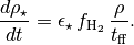
$\frac{d\rho_\star}{dt} = \epsilon_\star \, f_{\rm H_2} \, \frac{\rho}{t_{\rm ff}}.$

The SF time scale is the gas free fall time ( $t_{\rm ff} \sim \rho^{-1/2}$ ), and thus the SFR density is effectively proportional to $\rho^{3/2}$ . $\epsilon_\star$ (H2StarMakerEfficiency) is the specific star formation efficiency per free-fall time, which typically is around 1% (KT07). The SFR is proportional to the molecular hydrogen density, not the total gas density. The H₂ fraction ( $f_{\rm H_2}$ ) is estimated using the prescription given by KMT09 and MK10, which is based on 1D radiative transfer calculations and depends on the neutral hydrogen number density, the metallicity, and the H₂ dissociating flux. The prescription can be written down in four lines:

$\chi &= 71 \left( \frac{\sigma_{d,-21}}{R_{-16.5}} \right) \frac{G_0'}{n_H}; \qquad {\rm [MK10 \; Eq.(9)]} \\ \tau_c &= 0.067 \, Z' \, \Sigma_H; \qquad {\rm [KMT09 \; Eq.(22)]} \\ s &= \frac{ \ln( 1 + 0.6 \, \chi + 0.01 \, \chi^2)}{0.6 \tau_c}; \qquad {\rm [MK10 \; Eq.(91)]} \\ f_{\rm H_2} &\simeq 1 - \frac{0.75 \, s}{1 + 0.25 s} \qquad {\rm [MK10 \; Eq.(93)]}$

$\left( \frac{\sigma_{d,-21}}{R_{-16.5}} \right)$ is the ratio of the dust cross section per H nucleus to 1000 Angstroem radiation normalized to 10^-21 cm² ( $\sigma_{d,-21}$ ) to the rate coefficient for H₂ formation on dust grains normalized to the Milky Way value of 10^-16.5 cm³ s^-1 ( $R_{-16.5}$ ). Both are linearly proportional to the dust-to-gas ratio and hence the ratio is likely independent of metallicity. Although its value is probably close to unity in nature (see discussion in KMT09), Krumholz & Gnedin (2011) argue that in simulations with spatial resolution of ~50 pc, the value of $R_{-16.5}$ should be increased by a factor of ~30 in order to account for the subgrid clumping of the gas. The value of this ratio can be controlled with the parameter H2StarMakerSigmaOverR.
$G_0'$ is the H₂ dissociating radiation field in units of the typical value in the Milky Way (7.5x10^-4 cm³ s^-1, Draine 1978). At the moment only a spatially uniform and time-independent radiation field is supported, and its strength is controlled by the parameter H2StarMakerH2DissociationFlux_MW.
$Z'$ is the gas phase metallicity normalized to the solar neighborhood, which is assumed to be equal to solar metallicity: Z’ = Z/0.02.
$\Sigma_H$ is the column density of the gas on the scale of a giant atomic-molecular cloud complexes, so ~50-100 pc. This column density is calculated on the MaximumRefinementLevel grid cells, and it implies that this star formation method can only safely be used in simulations with sub-100pc resolution. If H2StarMakerUseSobolev is set, the column density is calculated through a Sobolev-like approximation,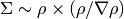 $\Sigma \sim \rho \times (\rho / \nabla \rho)$ , otherwise it’s simply $\Sigma = \rho \times dx$ , which introduces an undesirable explicit resolution dependence.
If H2StarMakerAssumeColdWarmPressureBalance == 1, then the additional assumption of pressure balance between the Cold Neutral Medium (CNM) and the Warm Neutral Medium (WNM) removes the dependence on the H₂ dissociating flux (KMT09). In this case

$\chi = 2.3 \left( \frac{\sigma_{d,-21}}{R_{-16.5}} \right) \frac{1 + 3.1 \, Z'^{0.365}}{\phi_{\rm CNM}}, \qquad {\rm [KMT09 \; Eq.(7)]}$

where $\phi_{\rm CNM}$ is the ratio of the typical CNM density to the minimum density at which CNM can exist in pressure balance with WNM. Currently $\phi_{\rm CNM}$ is hard-coded to the value of 3.

It is possible to impose an H₂ floor in cold gas, which might be applicable for some low density situations in which the KMT09 equilibrium assumption may not hold. The parameter H2StarMakerH2FloorInColdGas can be used to enforce such a floor for all cells that have temperature less than H2StarMakerColdGasTemperature. This has not been extensively tested, so caveat emptor.

Optionally, a proper number density threshold (H2StarMakerNumberDensityThreshold) and/or an H₂ fraction threshold (H2StarMakerMinimumH2FractionForStarFormation) is applied, below which no star formation occurs.

Typically this method is used with StarFormationOncePerRootGridTimeStep, in which case SF occurs only at the beginning of the root grid step and only for grids on MaximumRefinementLevel, but with a star particle mass that is proportial to the root grid time step (as opposed to the much smaller time step of the maximally refined grid). This results in fewer and more massive star particles, which improves computational efficiency. Even so, it may be desirable to enforce a lower limit to the star particle mass in some cases. This can be done with the parameter H2StarMakerMinimumMass, below which star particles are not created. However, with H2StarMakerStochastic, if the stellar mass is less than H2StarMakerMinimumMass, then a star particle of mass equal to H2StarMakerMinimumMass is formed stochastically with a probability of (stellar mass)/H2StarMakerMinimumMass.

Important Note: There is no feedback scheme corresponding to this star maker, so don’t set StarParticleFeedback = 2048. Instead the user should select one of the feedback schemes associated with the other star makers (StarParticleFeedback = 4 comes to mind).

Method 14: Kinetic Feedback¶

Select this method by setting StarParticleCreation = 16384 and StarParticleFeedback = 16384.

Source: star_maker3mom.F

This method combines stochastic Cen & Ostriker star formation (method 1) with a method for injecting both kinetic and thermal feedback energy into the grid.

The star formation method is identical to method 1, which supplements the star formation perscripton of Cen & Ostriker (1992) with a stochastic star formation recipe. Like method 1, there is no Jeans instability check, however, unlike method 1, the particle velocity is set to the gas velocity.

This star feedback method is described fully in Simpson et al. (2015) (S15). Feedback energy, mass and metals are injected into a 3x3x3 CIC stencil cloud that is centered on the particle position and mapped onto the physical grid. The outer 26 cells of the cloud stencil impart kinetic energy to the physical grid. The amount of momentum injected into each cell is computed assuming a fixed budget of kinetic energy and the direction of the injected momentum is taken to point radially away from the star particle.

CIC stencil overlap with the physical grid. The direction of imparted momentum is indicated with arrows. [Figure 1 S15]

As with methods 0 and 1, the total amount of feedback energy injected into the grid in a given timestep is

M_form * c² * StarEnergyToThermalFeedback

This energy is divided between thermal and kinetic energies. This is despite the name of StarEnergyToThermalFeedback, which would indicate that it is just thermal energy. This name was kept for consistency with other star makers.

If StarMakerExplosionDelayTime is negative, M_form is computed as it is for star maker methods 0 and 1 as described above. If StarMakerExplosionDelayTime >= 0.0 then M_form is the initial star particle mass. In this case, all energy, mass and metals are injected in a single timestep that is delayed from the formation time of the star particle creation by the value of StarMakerExplosionDelayTime, which is assumed to be in units of Myrs. When the feedback is done in a discrete explosion, the star particle field called dynamical_time is instead used as a binary flag that indicates wheter the particle has done its feedback or not (it is set to 1 pre-explosion and 0 once the explosion has been done). When StarMakerExplosionDelayTime < 0.0, dynamical_time has its usual meaning.

The amount of energy that takes kinetic form is fixed to be

M_form * c² * StarEnergyToThermalFeedback * f_kin

If StarFeedbackKineticFraction is between 0.0 and 1.0, f_kin = StarFeedbackKineticFraction. If StarFeedbackKineticFraction < 0.0, then f_kin is variable and depends on the gas density, metallicity and resolution surrounding the star particle at the time of the injection. Equations (16), (17) and (18) in S15 describe how this variable fraction is computed.

The injection of mass and metals is distributed evenly over the CIC stencil cloud and is done in proportion to M_form as described in method 0. The same parameters that control the mass and yield of ejected material are the same (i.e. StarMassEjectionFraction and StarMetalYield).

The discrete explosion mode and the variable kinetic energy injection mode are intended for use with low mass star particles which produce energy equivalent to only one or a few supernovae.

Restarting a Simulation With Star Formation or Feedback¶

Sometimes it is convenient to run a simulation for a while until it comes to some sort of equilibrium before turning on star formation.

If a simulation is initialized with star formation and feedback turned off, particles in the simulation will not have the necessary particle attribute fields Enzo uses to track data like the formation time, dynamical time, and metallicity.

To restart a simulation including star formation or feedback, simply edit the parameter file written to disk in the data dump folder (i.e. for a dataset named DD0100, the parameter file will typically be named DD0100/DD0100. Change the parameters StarParticleCreation or StarParticleFeedback to the values needed for your simulation, and restart the simulation. Enzo will detect that it needs to create particle attribute fields and allocate the necessary memory above what is needed to read in the dataset.

Distributed Stellar Feedback¶

The following applies to Methods 0 (Cen & Ostriker) and 1 (+ stochastic star formation).

The stellar feedback can be evenly distributed over the neighboring cells if StarFeedbackDistRadius > 0. The cells are within a cube with a side StarFeedbackDistRadius+1. This cube can be cropped to the cells that are StarFeedbackDistCellStep cells away from the center cell, counted only in steps in Cartesian directions. Below we show a couple of two-dimensional examples. The number on the cells indicates the number cell steps each is from the central cell.

StarFeedbackDistRadius = 1

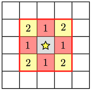
Only cells with a step number <= StarFeedbackDistCellStep have feedback applied to them. So, StarFeedbackDistCellStep = 1 would result in only the cells marked with a “1” receiving energy. In three-dimensions, the eight corner cells in a 3x3x3 cube would be removed by setting StarFeebackDistCellStep = 2.

StarFeedbackDistRadius = 2

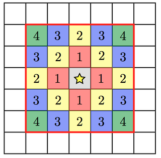
Same as the figure above but with a radius of 2.

Feedback regions cannot extend past the host grid boundaries. If the region specified will extend beyond the edge of the grid, it is recentered to lie within the grid’s active dimensions. This conserves the energy injected during feedback but results in the feedback sphere no longer being centered on the star particle it originates from. Due to the finite size of each grid, we do not recommend using a StarFeedbackDistRadius of more than a few cells.

Also see Star Formation and Feedback Parameters.

Notes¶

The routines included in star_maker1.F are obsolete and not compiled into the executable. For a more stable version of the algorithm, use Method 1.

Active Particle Framework¶

To be added.

Magnetic Supernova Feedback¶

Source: hydro_rk/SuperNovaSeedField.C

Select this method by setting UseMagneticSupernovaFeedback = 1 (Default = 0) and specifying the parameters below. If UseMagneticSupernovaFeedback == 2, the parameters MagneticSupernovaRadius and MagneticSupernovaDuration will be calculated to be the minimum allowed values (see below) at runtime based on the cell width and time step of the most-refined grid.

MagneticSupernovaEnergy (in units of ergs) is the total amount of magnetic energy to be injected by a single supernova event. Defualt = 1e51 ergs.

MagneticSupernovaRadius (in units of parsecs) gives the scale over which to inject supernova energy. The injection mechanism normalizes the spatial exponential decay of the injected supernova energy so that all of the energy is contained within the specified radius. For this reason, the MagneticSupernovaRadius should be at least 1.5 times the minimum cell width of the simulation (in pc). Default = 300 pc.

MagneticSupernovaDuration (in units of years) gives the duration of the supernova magnetic energy injection. The injection mechanism is normalized so that all of the MagneticSupernovaEnergy is injected over this time scale. In order to inject the correct amount of energy, MagneticSupernovaDuration should be set to at least 5 times the minimum time step of the simulation. Default = 50,000 years.

The following applies to all star formation methods that produce a PARTICLE_TYPE_STAR object. Methods 0 (Cen & Ostriker) and 1 (+ stochastic star formation) have been tested extensively. The magnetic feedback method is described fully in Butsky et al. (2017).

When a star cluster particle reaches the end of its lifetime, we inject a toroidal loop of magnetic field at its position in hydro_rk/Grid_MHDSourceTerms. The spatial and temporal evolution of the injected magnetic energy and magnetic field is chosen to be:

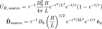
$\dot{U}_{B,\, {source}} = \tau^{-1} \frac{B_0^2}{4\pi} \frac{R}{L} e^{-r^2/L^2} e^{-t/\tau} (1-e^{-t/\tau})\\ \mathbf{\dot{B}}_{source} = \tau^{-1} B_0 \left(\frac{R}{L}\right)^{1/2} e^{- r^2 / 2L^2} e^{-t / \tau} \, \hat{\mathbf{e}}_\phi$

where t is the time since the ‘death’ of the star cluster particle, $\tau$ is the SupernovaSeedFieldDuration, R is the cylindrical radius, r is the spherical radius, and L is the SupernovaSeedFieldRadius.

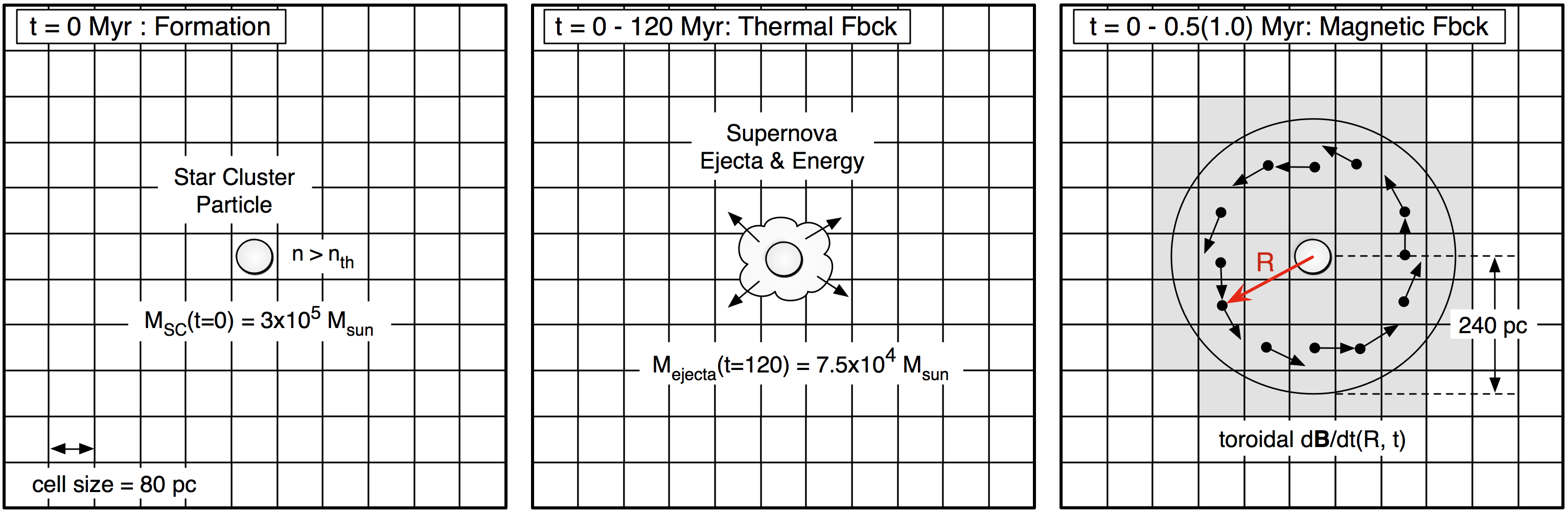
Two-dimensional schematic overview of the life cycle of a star cluster particle and two channels of its feedback. Left: Star cluster particle formation. Middle: Thermal feedback. Thermal energy by Type II supernova explosion is injected into the gas cell in which a star cluster particle of age less than 120 Myr resides. Right: Magnetic feedback. Toroidal magnetic fields are seeded within three finest cells from a star cluster particle.

Enzo 2.6 documentation