MHD Methods
Dedner cleans  with a wave-like hyperbolic cleaner, and is
easy to use.
with a wave-like hyperbolic cleaner, and is
easy to use.
CT preserves to machine precision, but is slightly harder to use.
quantity MHD-RK MHD-CT/MHD_Li Reconstruction PLM PLM Splitting Unsplit, Runge Kutta Split (strang) Few Percent Machine Noise Difficulty Easy Two pitfalls
Use of Dedner
The Dedner method (HydroMethod = 4) is relatively straight forward.
The three magnetic components are stored in BaryonField, with the relevant
indices found through IdentifyFieldQuantities. Since they hyperbolic
cleaner will largely eliminate any divergence, initialization an injection of
magnetic energy is straight forward.
AMR is done in the same manner as other fluid quantities in Enzo.
The method is described in Dedner et al. 2002 JCP 175, 2, 645-673
The implementation and test problems can be found in Wang & Abel 2009, ApJ 696 96.
Use of MHD-CT
Use of MHD-CT (HydroMethod = 6) is somewhat complicated by the staggered nature of the magnetic field. This allows the
field to be updated by the curl of an electric field, thus preserving
 to machine precision, but requires some additional
machinery to ensure consistency of the data structure. In principle,
Constrained Transport can be used with a variety of MHD methods, but presently
it only works with the second-order scheme described by Li, Li, and Cen. For
this reason, a distinction is made between the hydro solver,
to machine precision, but requires some additional
machinery to ensure consistency of the data structure. In principle,
Constrained Transport can be used with a variety of MHD methods, but presently
it only works with the second-order scheme described by Li, Li, and Cen. For
this reason, a distinction is made between the hydro solver, MHD_Li as it is
referred to in the code, and CT.
The magnetic field is represented by two data structures.
- The cell centered magnetic field is accessed the same manner as done in
HydroMethod==4. However, this is a read only quantitiy. Periodically it is replaced by the spatial average of the face centered magnetic field. - The face centered magnetic field is stored in
MagneticField. This is a staggered structure, and is divergence free. If a modification need to be made to the magnetic field when using MHDCT (such as injection by a source or initialization), the modification should be done in a divergence free manner. More details below.
The primary references are:
CT algorithms: Balsara & Spicer 1999, JCP, 149, 2, 270-292
Gardiner & Stone 2005, JCP, 205, 2, 509-539
AMR Algorithm: Balsara 2001 JCP, 174, 2, 614-648
Implementation and test problems: Collins, Xu, Norman, Li & Li, ApJS 186, 2, 308.
Controlling MHD in the code
Within the code, there are several flags to control use of magnetic fields.
UseMHD is true when either MHD module is on.
UseMHDCT controls use of the face- and
edge- centered fields. While it is associated with HydroMethod=6, in
it only controlls the face- and edge-centered fields, so future HydroMethods
can also use these fields.
HydroMethod==MHD_RK controls things that only pertain
to that hydro method. This is either control of the solver itself, or the
fields that pertain exclusively to that solver
(e.g. BaryonField[PhiNum], the Phi field is exclusive to the Dedner method.)
HydroMethod==6 or HydroMethod==MHD_Li typically only deals with control of the MHD_Li solver. Currently this only triggers the call to the solver. Things dealing with the data structures should be controlled with UseMHDCT
Wait, what? UseMHD is usually what you want to use in your code. UseMHDCT is for
MagneticField or ElectricField. HydroMethod==MHD_RK when you need
the Phi field, which you only really need for initialization.
Implementation details for MHDCT can be found in MHDCT Details
Cosmology
As of January 2015, the cosmology has been modified slightly in MHDCT. This was
done in order to rectify the treatment of cosmology in the bulk of the code as
well as the output fields, and to rectify a missing  in the pressure
when using MHDCT (it probably did not impact your run.) For clarity we briefly
summarize the differences here. The major difference between
in the pressure
when using MHDCT (it probably did not impact your run.) For clarity we briefly
summarize the differences here. The major difference between MHD_RK and
MHD_Li is now the treatment of the dilution of the field due to cosmological
expansion. These terms are the  in the method papers.
In both methods, the magnetic field most often seen in the code and in output is
the comoving magnetic field. The induction equation for the comoving magnetic
field has an expansion term,  . For
. For MHD_RK, this is
integrated in Grid_MHDSourceTerms.C, by way
of direct finite difference. For MHDCT, the induction is formulated with a
semi-comoving field, 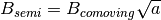 . In this
formulation there is no explicit expansion source term. This is done in order
to keep the divergence zero, and is the result of the manner in which
projection from fine to coarse grids happens in the code. In order to keep the
code representation consistent throughout the bulk of Enzo, this change of
fields from comoving to semi-comoving is done in
. In this
formulation there is no explicit expansion source term. This is done in order
to keep the divergence zero, and is the result of the manner in which
projection from fine to coarse grids happens in the code. In order to keep the
code representation consistent throughout the bulk of Enzo, this change of
fields from comoving to semi-comoving is done in
Grid_MHD_UpdateMagneticField.C. It should be noted that in the Bryan et al
2014, the total pressure is stated as 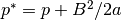 (Equation 6 in
that paper.) This is no
longer valid, now the total pressure should be
(Equation 6 in
that paper.) This is no
longer valid, now the total pressure should be 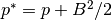 for both
solvers in both the code and in analysis.
for both
solvers in both the code and in analysis.
It should also be noted that ElectricField is semi-comoving.
Care should be taken with simulations using cosmology and MHDCT that were
run before Fall 2015.